The components of the simulation

The two main components of the simulation are the Geometry and Physics providing information and functionalities required to compute the individual simulation steps during the Event processing inside the Stepping loop. The information is fused together in order to calculate how far the particle goes in a given step and what happens with it both along its way to and at the corresponding post-step point.

The Geometry describes the simulation setup, including navigation possibilities or providing information on the geometrical constraints for the simulation step computation (e.g. given a global point, how far the nearest volume boundary is or how far the volume boundary to a given direction is, etc.). The Physics component is responsible to supply the physics related constraints for the simulation step computation (e.g. how far the given particle go till its next interaction of the given type or how far a charge particle goes till it loses all its current energy, etc.). These constraints are required during the Event processing at the beginning of each simulation step computation in the Stepping loop to decide length of the simulation step. The particle is then moved to the post-step point and the necessary Geometry and/or Physics related actions are performed on the particle. Some information regarding the given simulation step, e.g. energy deposit, might be collected at the end of each simulation step before performing the computation of the next step till the history of the particle is terminated (e.g. \(e^-\) lost all its kinetic energy in the last step; \(\gamma\) was absorbed in photoelectric process or destructed by producing \(e^-/e^+\) pair, etc.).

While the above components perform the event processing, the smaller Primary generator simulation component is used to generate primary particle track(s) at the beginning of each event. Further, auxiliary components, like the Input arguments or the Results are also added to complete the simulation by providing configuration options and the possibility of collecting some (even more) application specific data during the simulation.

A short description of these components is provided in this section together with the The HepEmShow application main.

Geometry

The application Geometry is a configurable simplified sampling calorimeter that is built up from N layer-s of an absorber and a gap as illustrated in Fig. 1.

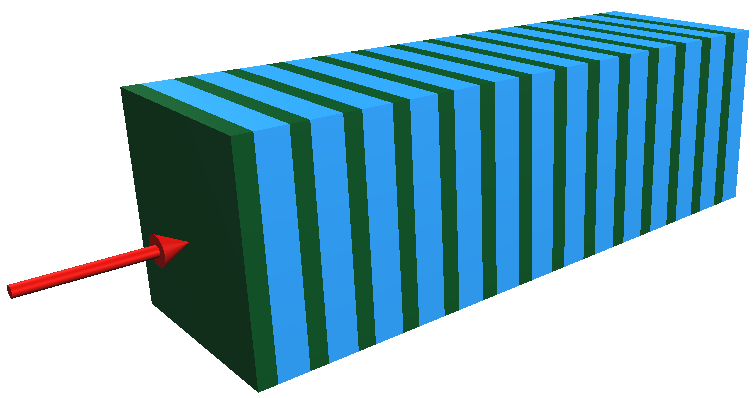
geom-calo_layer2 — Fig. 1 Illustration of the default `absorber` (green) and `gap` (blue) `layer` structured simplified sampling calorimeter configuration (with `N = 14` `layer`-s in this case). The red arrow from left represents the direction of the incoming primary particle beam.

The number of layer-s N, the thickness of both the absorber and gap can be set at the construction of the calorimeter (see the Input arguments of The HepEmShow application main). All thicknesses are measured along the x-axis in mm units.

Note

The gap thickness can be set even to zero in which case the calorimeter is built up from the given number of layer-s of absorber with the given thickness (i.e. a single material calorimeter sliced by the layer-s) as illustrated in Fig. 2.

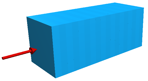
geom-calo_layer1 — Fig. 2 Illustration of the single material calorimeter sliced by the `layer`-s (`N = 18`). As the `gap` thickness is set to `0`, the single `layer` thickness is identical to the `absorber` (blue) thickness while the `calorimeter` thickness is \(\times\) `N` of that.

The thickness of the single layer as well as the entire calorimeter is automatically computed from the given absorber, gap thicknesses and number of layer-s respectively. The transverse size, i.e. the full extent of the absorber, gap, layer and the calorimeter along the y- and z-axes, can also be set as an input argument (see the Input arguments of The HepEmShow application main). The calorimeter is places in the center of the world so 5 (Box shaped) volumes are used in total to describe the application geometry. The size of the world volume is computed automatically based on the extent of the calorimeter such that it encloses the entire calorimeter with some margin.

Note

The x-coordinate of the left hand side boundary of the calorimeter as well as an appropriate initial x-coordinate of the primary particles (such that they are located mid-way between the calorimeter and the world boundaries along the negative x-axis) are calculated. At the beginning of an event, the PrimaryGenerator will generate primary particles at this later position with the [1,0,0] direction vector, i.e. pointing toward to the left hand side boundary of the calorimeter. Each primary particle is then moved to the former position, i.e. on the left hand side boundary of the calorimeter, in their very first step such that they will enter into the calorimeter in the next, second simulation step.

Each of these volumes is filled with a given material specified by the material index of the volume. These indices are the subscripts of the (Geant4 predefined NIST) materials listed in the material name vector of The HepEmShow-DataGeneration application main. In the default case, which is the same that was used to generate the G4HepEm data shipped with the application, this material name vector is

Listing 1 The material name vector as it is in The HepEmShow-DataGeneration application main.

// list of Geant4 (NIST) material names
std::vector<std::string> matList {"G4_Galactic", "G4_PbWO4", "G4_lAr"};

This corresponds to the default index-to-material and eventually to the material-to-volume association shown in Table 1. A complete list of the predefined NIST materials provided by Geant4 with their composition can be found at the corresponding part of the Geant4 documentation (Book For Application Developers: Geant4 Material Database).

Table 1 The default material to index and material to volume association.
Material	Index	Used in Volume
galactic (low density gas)	0	`layer` `calorimeter` `world`
lead tungstate (atolzite)	1	`absorber`
liquid-argon	2	`gap`

Note

Changing the material name(s) in this above vector of the The HepEmShow-DataGeneration application main (especially at index 1 and/or 2 as the vacuum is always needed to fill the layer, calorimeter and world container volumes), regenerating the data by executing this data generation application, then executing again the HepEmShow application, corresponds to changing the material of the absorber and/or gap volumes of the simulation.

The application geometry also provides a rather simple “navigation” capability (used in the simulation stepping loops) through its Geometry::CalculateDistanceToOut() method described in details at the corresponding code documentation.

Attention

Unlike the Geant4 geometry modeller and navigation, that provides generic geometry description and navigation capabilities, the Geometry implemented for HepEmShow is specific to the configurable simplified sampling calorimeter described above. Focusing only to this specific geometry modelling and related navigation problem made possible to provide a rather compact, simple and clear implementation of all geometry related functionalities required during the simulation (i.e. in the SteppingLoop).

Physics

Targeting only the simulation of the EM shower inherently leads to a compact simulation as it includes only \(e^-/e^+\) and \(\gamma\) particles with their EM (i.e. without gamma- and lepto-nuclear) interactions. Focusing to the descriptions of these interactions, that ensures sufficient details and accuracy for HEP detector simulations, leads to an even more specific set of interactions and underlying models that the physics component of the simulation needs to provide. This well defined, important but small subset of the very rich physics offered by the Geant4 toolkit, can then be implemented in a very compact form.

The G4HepEm R&D project [4] offers such an implementation with several attractive properties. Separation of data definition, initialisation and run-time functionalities results in a rather small, Geant4 independent, stateless, header based implementation of all physics related run-time functionalities required for such EM shower simulations. Furthermore, all the data, extracted from Geant4 during the initialisation, can be exported/imported into/from a single file making possible to skip the Geant4 dependent initialisation phase in subsequent executions of the application. Therefore, G4HepEm offers the possibility of a Geant4 like but Geant4 independent EM physics component for developing particle transport simulations. Further information on G4HepEm, including the physics interactions included, can be found in the corresponding part of the G4HepEm documentation.

Note

The hepemshow repository includes the pre-generated data file (/data/hepem_data.json) that has been extracted by using the HepEmShow-DataGeneration with the default material configuration settings. Providing this data file makes possible to initialise the G4HepEm data component from this file making HepEmShow independent from Geant4. The HepEmShow-DataGeneration application is also available in the hepemshow repository. This can be used to re-generate the above data file when the goal is to change the default material configuration (see above at the Geometry section). However, as the data extraction requires the Geant4 dependent initialisation of G4HepEm, it requires a Geant4 dependent build of G4HepEm. See more details in the Build and Install section.

As mentioned above, the entire physics of the HepEmShow simulation application is provided by G4HepEm [4]. The required, definitions (.hh files) of the G4HepEm run-time functionalities are pulled in by the Physics.hh header while the corresponding implementations (.icc files) are in the Physics.cc. The only missing implementation, that the client needs to provide, is a uniform random number generator that needs to be utilised to complete the implementation of the G4HepEmRandomEngine. This is also done in the Physics.cc file by using the local URandom uniform random number generator. More information can be found in the code documentation of the Physics.

G4HepEm provides two top level methods, HowFar and Perform in its G4HepEmGammaManager and G4HepEmElectronManager for \(\gamma\) and \(e^-/e^+\) particles respectively:

HowFar: the physics constrained step length of the given input track, i.e. how far the particle goes e.g. till the next physics interaction takes place or it loses all its kinetic energy or due to any other physics related constraints.

Perform: performs all necessary physics related actions and updates on the given input track, including the production of secondary tracks in the given physics interaction (if any).

These two top level methods are utilised in the Stepping loop during the computation of the individual simulation step. HowFar is invoked at the pre-step point, i.e. at the step limit evaluation, while Perform is utilised at the post-step point of each individual simulation step computation inside the SteppingLoop::GammaStepper() and SteppingLoop::ElectronStepper() methods.

Attention

Unlike the Geometry of the application, the Physics is fully generic as G4HepEm provides an application independent, generic EM physics component similarly to the corresponding native Geant4 implementation. However, the Geant4 dependent initialisation phase of G4HepEm, i.e. the data extraction, has been eliminated from HepEmShow by separating it to the additional HepEmShow-DataGeneration application in order to make HepEmShow independent from Geant4. As a consequence, the corresponding generated data file is specific to a given material configuration and needs to be re-generated whenever one would like to change that material configuration as discussed above.

Primary generator

The primary generator is used to:

store the properties of the primary particle track

generate such primary particle tracks to initiate a new event

The properties of the primary generator can be set by providing the appropriate Input arguments when executing the HepEmShow simulation application. The PrimaryGenerator::GenerateOne() method is invoked then from the Event loop at the beginning of each event to generate a primary particle track.

Note

An event is assumed to be composed form a single primary particle track but only for simplicity as most of the event processing would work fine with more than one primary tracks as well.

Event processing

After reading the Input arguments and setting up the Physics, Geometry and Primary generator components accordingly, the HepEmShow simulation is ready for event processing. The event processing consists of an outer Event loop, a small intermediate tracking loop and the innermost Stepping loop.

The Event loop is running over the individual events and responsible for generating and initialising a track stack with the corresponding primary particle track. The intermediate small tracking loop just takes the next track from this stack and invokes the appropriate Stepping loop. The entire history of the inserted track is simulated then by this innermost loop, including generation of secondary particle tracks (also inserted into the track stack for later tracking), in a step-by-step way.

The simulation of a particle history is terminated when the particle kinetic energy goes to zero, undergoes a destructive interaction or simple leaves the simulation setup. As long as the stack is not empty, a new track is taken and its history is simulated similarly while the simulation of the actual event is completed otherwise. As long as the number of simulated events is less than the required, a new event is generated and its processing starts similarly while the simulation is completed otherwise.

Event loop

The event loop is responsible for the generation and simulation of the required number of primary events.

At the beginning of each event, the Primary generator is invoked to produce the actual event, i.e. the primary particle track (one primary per event for simplicity) that belong to the actual event. The generated primary track is inserted/pushed into the TrackStack as the very first track and the simulation of the event starts. During the simulation of the event:

one track is popped from the stack

inserted in the appropriate Stepping loop to simulate its entire history in a step-by-step way (see below)

At the end of each simulation step, secondary tracks that are created in that step in the related physics interaction (if any), are inserted/pushed into the TrackStack. At the beginning of a typical EM shower, the TrackStack is growing as usually more than one secondary is created per history. This will start to shrink then when popping up more and more low energy particles that do not produce any secondaries in their history. The simulation of the event is then completed when the TrackStack becomes empty again. A new event might be generated at this point till the requested number of simulated event is reached when the simulation terminates.

In order to provide the possibility of interacting with the simulation at the event and stacking level, e.g. for collecting some information during the event processing or stacking, the EventLoop::BeginOfEventAction() / EventLoop::EndOfEventAction() methods are invoked before/after each event processing while the EventLoop::BeginOfTrackingAction() / EventLoop::EndOfTrackingAction() methods are invoked before/after tracking each new track.

A typical task that is done at the beginning of a new event is to clear/reset some variables that will be used then during the processing of the event to accumulate information like the total energy deposited during the given event in the absorber. At the end of the event, the collected information might be stored at or added to a higher, i.e. entire simulation, level. A typical task that can be done at the beginning of tracking is to inspect the properties of a particle before inserting to the Stepping loop. Moreover, even the behaviour can be changed by altering some of the particle properties, e.g. setting its kinetic energy to zero discards the particle from tracking as the Stepping loop terminates immediately.

More details can be found by inspecting the implementation of the EventLoop::EventProcessing() method.

Stepping loop

Stepping loops can calculate a given \(\gamma\) (SteppingLoop::GammaStepper()) or \(e^-/e^+\) (SteppingLoop::ElectronStepper()) particle simulation history from the initial state of the particle track, i.e. as inserted from the Event loop, till the end in a step-by-step way. At each step:

the actual step length is calculated, accounting both the Geometry and the Physics related constraints

the track is moved to its post-step position

all physics related actions, happening along and/or at the post-step point, are performed on the track

secondary tracks, generated in the given step by a physics interaction (if any), are inserted into the track stack

In order to provide the possibility of interacting with the simulation at the end of each simulation step, the SteppingLoop::SteppingAction() method is invoked. This can be used to e.g. obtain information on the energy deposited in the given simulation step.

The particle simulation history is terminated when either:

the particle kinetic energy becomes zero (e.g. an \(e^-\) lost all its kinetic energy in its last step)

the particle participated in a destructive interaction (e.g. photoelectric absorption of a \(\gamma\) photon or conversion to \(e^-/e^+\) pairs)

the particle leaves the calorimeter (in a normal Geant4 simulation this would happen when the particle leaves the world but in our case that would be just one more step in vacuum)

More details can be found by inspecting the implementation of the SteppingLoop::GammaStepper() and SteppingLoop::ElectronStepper() methods.

Attention

The event processing algorithm, including both the Event loop and Stepping loop, is general, i.e. not application specific as long as the geometry related methods provide the expected behaviour. However, the event, tracking and stepping actions are rather specific to the (implemented simplified sampling calorimeter) simulation application as they implement the application specific information extraction. This is exactly the same with a pure Geant4 simulation application as the corresponding user actions are implemented for and thus specific to a given simulation application while the entire event processing loop is part of the generic, internal Geant4 simulation kernel.

Additional components

While Geometry, Physics, Primary generator and the Event processing are essential components of any simulations, the additional Input arguments and Results are used to provide configuration options to them and the possibility of collecting some (even more) application specific data during the simulation respectively.

Input arguments

The InputParameters can be used to set some Geometry, Physics, Primary generator and Event processing related parameters of the HepEmShow simulation application. The configurable parameters, with their default values, are reported when executing the simulation application as:

$ ./HepEmShow --help

=== Usage: HepEmShow [OPTIONS]

   -l  --number-of-layers      (number of layers in the calorimeter)           - default: 50
   -a  --absorber-thickness    (in [mm] units)                                 - default: 2.3
   -g  --gap-thickness         (in [mm] units)                                 - default: 5.7
   -t  --transverse-size       (of the calorimeter in [mm] units)              - default: 400
   -p  --primary-particle      (possible particle names: e-, e+ and gamma)     - default: e-
   -e  --primary-energy        (in [MeV] units)                                - default: 10 000
   -n  --number-of-events      (number of primary events to simulate)          - default: 1000
   -s  --random-seed                                                           - default: 1234
   -d  --g4hepem-data-file     (the pre-generated data file with its path)     - default: ../data/hepem_data
   -v  --run-verbosity         (verbosity of run information: nothing when 0)  - default: 1
   -h  --help

or with the actual values when executing a simulation application as:

$ ./HepEmShow  --number-of-layers 42  --primary-energy 200

  === HepEmShow input parameters:
      --- Geometry configuration:
          - number-of-layers      : 42
          - absorber-thickness    : 2.3 [mm]
          - gap-thickness         : 5.7 [mm]
          - transverse-size       : 400 [mm]
      --- Primary and Event configuration:
          - primary-particle      : e-
          - primary-energy        : 200 [MeV]
          - number-of-events      : 1000
          - random-seed           : 1234
      --- Additional configuration:
          - g4hepem-data-file    : ../data/hepem_data.json
          - run-verbosity        : 1
  --- EventLoop::ProcessEvents: starts simulation of N = 1000 events...

Results

Results is a simply data structure that can be used to collect information during the event processing. These information can be updated in the provided action methods that offer the possibility of interacting with the simulation at the different point of the event processing (outer, immediate and inner loops):

event: EventLoop::BeginOfEventAction() / EventLoop::EndOfEventAction() invoked before/after processing and event

tracking: EventLoop::BeginOfTrackingAction() / EventLoop::EndOfTrackingAction() invoked before/after simulating the history of a track

stepping: SteppingLoop::SteppingAction() invoked after each individual simulation steps

The Results data structure is used to collect the following information during the event processing (by default):

mean values of energy deposit, neutral (gamma) and charged (electron/positron) particle track length per event in the individual calorimeter layers

mean number of energy deposited in the absorber and gap materials per event

mean number of secondary gamma, electron and positrons produced per event

mean number of neutral (gamma) and charged (electron/positron) steps pre event

Quantities, recorded in the individual layers are stored in histograms and written to files at the end of the simulation (see some Examples below) while others are reported by printing to the standard output as (default run):

--- Results::WriteResults ----------------------------------

Absorber: mean Edep = 6722.95 [MeV] and  Std-dev = 309.636 [MeV]
Gap     : mean Edep = 2571.75 [MeV] and  Std-dev = 118.507 [MeV]

Mean number of gamma       4457.043
Mean number of e-          7957.899
Mean number of e+          428.922

Mean number of e-/e+ steps 36097
Mean number of gamma steps 40436.2
------------------------------------------------------------

The `HepEmShow` application main

The above simulation components are fused together in the HepEmShow main function to form the corresponding simulation application with the following steps:

reads the Input arguments, provided at the execution of the application, that determines the actual configuration

Physics and the underlying G4HepEm related configuration steps:

initialising G4HepEm by loading the corresponding data and parameters from the pre-generated state file (can be set by the --g4hepem-data-file input argument)

constructs the additional G4HepEmTLData that encapsulates the (application local, uniform URandom based) random number generator as well as some track buffers. This is used in all information exchange between the underlying G4HepEm implementation of the physics and the simulation application

constructs and sets up the application Geometry according to the provided related input arguments

constructs and sets up the Primary generator of the application according to the provided related input arguments

constructs and sets up a Results structure that will be used to collect some data during the simulation

the Event processing is invoked then by calling the EventLoop::ProcessEvents() method with the provided related input arguments to perform the simulation

when completing the event processing, the simulation Results are written to files (histograms) and reported on the standard output when invoking WriteResults()

Examples

1. Simulation results compared to a Geant4 simulation:

The simplified sampling calorimeter application, implemented in HepEmShow can be found in the G4HepEm repository [4] as an example implemented as a Geant4 simulation application. This offers the possibility to compare the Geant4 independent HepEmShow simulation results to those obtained by the corresponding Geant4 based version of the simulation.

The default simulation configuration was used in this example with the only difference that the number of required events was set to \(10^7\) in order to reduce the statistical uncertainty. \(\texttt{TestEm3}\), the Geant4 based version as taken from the G4HepEm repository, was used by setting the geometry configuration identical to the default HepEmShow geometry. The physics component of the Geant4 based simulation was chosen to be the same as used in HepEmShow (i.e. G4HepEm). While G4HepEm can reproduce the corresponding native, Geant4 physics based results with an excellent precision (relative error within per mille), this setting ensures that only the HepEmShow locally implemented components (i.e. Geometry, Event processing, etc. everything than Physics) are different.

The mean energy deposit, obtained by using the default configuration of the Geant4 independent HepEmShow simulation, is compared to the corresponding result produced by the above-mentioned Geant4 based version of the application in Fig. 3 while the other observables are reported in Table 2. An excellent agreement can be seen that verifies the correct behaviour of all HepEmShow locally implemented components. It must be noted, that the somewhat larger (but still rather small) difference observed in the mean number of \(e^-/e^+\) steps is the effect of the slightly different multiple Coulomb scattering contribution to step limit (due to some difference in the geometry/navigation).

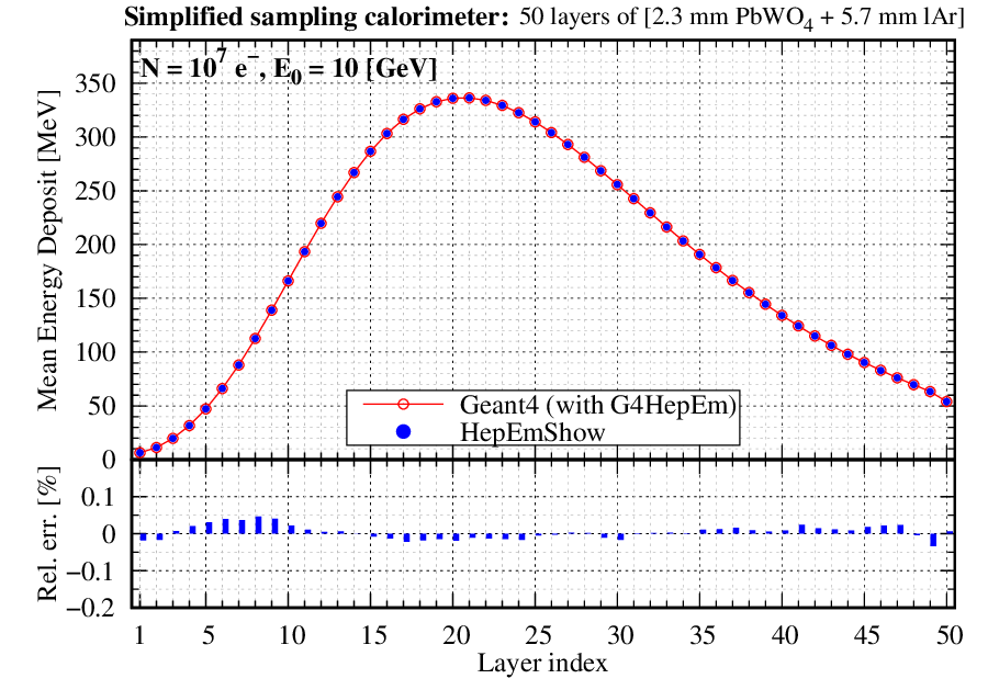
edep-hepemshow-vs-g4 — Fig. 3 Comparison of the mean energy, deposited in the individual calorimeter layers, obtained by `HepEmShow` and the corresponding `Geant4` based implementation of the same application.

Table 2 Summary of the simulation results obtained by `HepEmShow` and the corresponding `Geant4` based implementation of the same application. The reported mean energy deposited in the `absorber`/`gap` materials, mean number of produced secondaries as well as charged (i.e. \(e^-/e^+\)) and neutral (i.e. \(\gamma\)) simulation steps per event are in an excellent agreement.
		\(\texttt{Geant4}\)	\(\texttt{HepEmShow}\)	rel. error [%]
\(\text{E}_{\text{dep}}\) [MeV]	\(\texttt{PbWO}_4\)	6726.72	6726.78	-0.00089
\(\text{E}_{\text{dep}}\) [MeV]	\(\texttt{lAr}\)	2568.84	2568.89	-0.00195
#secondaries	\(\gamma\)	4458.02	4458.02	0
	\(e^-\)	7961.90	7962.06	-0.002
	\(e^+\)	429.309	429.314	-0.0011
#steps	\(\texttt{charged}\)	36238.1	36103.4	0.3717
#steps	\(\texttt{neutral}\)	40458.4	40458.2	0.00049

2. Simulation results obtained with different configurations:

Fig. 4 shows mean energy deposits (per event, as a function of the calorimeter layer index, i.e. depth) obtained by running the HepEmShow simulation with different absorber and gap thicknesses using the default \(E_0 = 10\) [GeV] \(e^-\) primary particles.

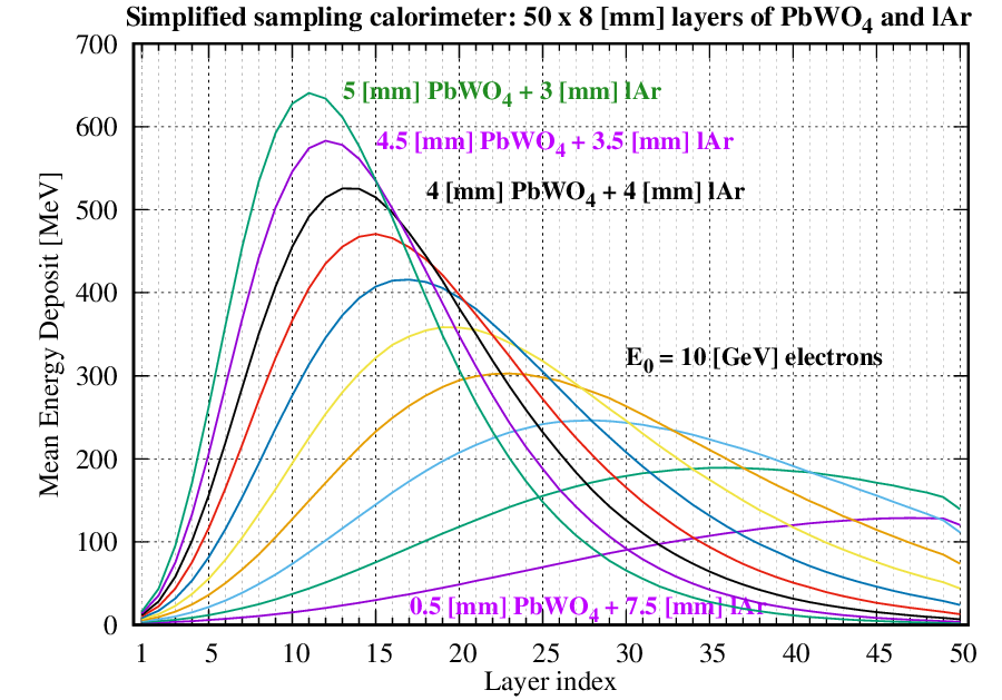
edep-hepemshow-8mm — Fig. 4 Variation of the mean energy deposit when changing the `absorber` and `gap` thickness of the layers such that the layer thickness as well as all other configurations are kept constants. The default \(E_0 = 10\) [GeV] \(e^-\) were used as primary events.

As an example, the result that corresponds to the 4.0 [mm] absorber (\(\texttt{PbWO}_4\)) and 4.0 [mm] gap (\(\texttt{lAr}\)) thickness run in Fig. 4 can be obtained by executing HepEmShow with the following parameters (all others stays default):

$ ./HepEmShow \
  --absorber-thickness 4.0 \
  --gap-thickness 4.0

The results shown in Fig. 5 were obtained by setting a 2.0 [mm] thickness for the absorber while zero for the gap. This corresponds to a Geometry of a single (\(\texttt{PbWO}_{4}\)) material sliced by 2.0 [mm] layers along the primary particle direction (see more at the Geometry). The number of layers was set to 200 and the results, obtained by varying the primary particle (\(e^-\)) energy between \(E_0 = [0.2 - 10]\) [GeV], are shown.

Fig. 5 shows mean energy deposits (per event, as a function of the calorimeter layer index, i.e. depth) obtained by running the HepEmShow simulation with different absorber and gap thicknesses using the default \(E_0 = [0.2 - 10]\) [GeV] \(e^-\) primary particles.

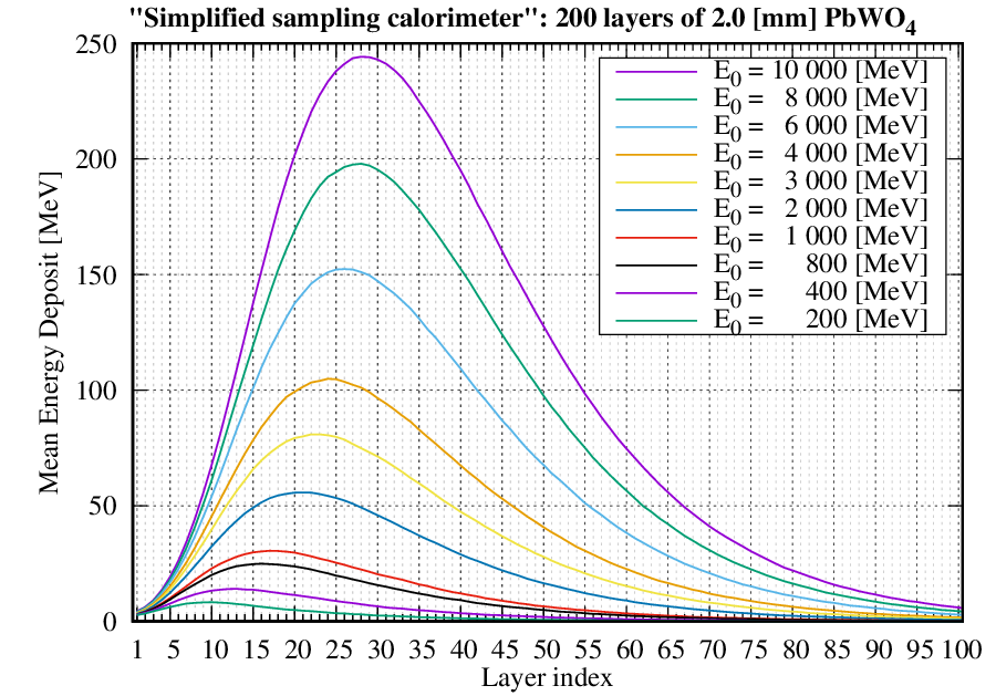
edep-hepemshow-edep — Fig. 5 Variation of the mean energy deposit, as a function of the depth (with a resolution/bin-with of 2.0 [mm]), when changing the primary particle (\(e^-\)) energy.

As an example, the result that corresponds to the \(E_0 = 2.0\) [GeV] run in Fig. 5 can be obtained by executing HepEmShow with the following parameters (all others stays default):

$ ./HepEmShow \
  --absorber-thickness 2.0 \
  --gap-thickness 0 \
  --number-of-layers 200 \
  --primary-energy 2000

The `HepEmShow-DataGeneration` application main

The physics of the HepEmShow simulation application is provided by G4HepEm. As mentioned at the Physics, Geometry or even in the Details subsection of the Build and Install sections, the Geant4 dependent initialisation part of G4HepEm is well separated from the rest. Furthermore, the already initialised state of G4HepEm, that depends on the material (and production cut) configuration of the application in hand, can be exported to a state file and G4HepEm can then be re-initialised solely from such a state file skipping the Geant4 dependent initialisation part. This is how G4HepEm provides a Geant4 independent physics component for EM shower simulations exploited in HepEmShow.

However, as the physics depends on the material (and secondary production threshold) configuration of the application geometry, a given state file corresponds to a given material (and cut) configuration of the application. The G4HepEm state file that corresponds to the default material configuration of the Geometry is available in the repository in order to be able to use the HepEmShow simulation application without Geant4 (but only with the default material configuration). The auxiliary HepEmShow-DataGeneration application, that was used to generate the G4HepEm state file, is also available for providing the possibility of changing this default material configuration (see Table 1) by generating new G4HepEm state files that correspond to different material configurations.

It must be noted though, that this HepEmShow-DataGeneration application requires both a Geant4 and a complete, Geant4 dependent build of G4HepEm installed on the system as both the application itself and the initialisation of G4HepEm (i.e. producing the state) depend on Geant4 (see more at the Build and Install sections).

The HepEmShow-DataGeneration application:

builds and pre-initialises a Geant4 geometry with the given list of materials (and secondary production threshold value) to be ready for the physics initialisation

initialises G4HepEm according to the geometry (material cut) configuration

exports the already initialised G4HepEm state to a file

The required materials are given as a vector of pre-defined Geant4 material names in the HepEmShow-DataGeneration application main. The material at index 1 corresponds to the absorber while the one at index 2 to the gap materials of the HepEmShow simulation application geometry. Therefore:

by editing the pre-defined Geant4 material name given in the HepEmShow-DataGeneration application main (the default is):
// list of Geant4 (NIST) material names
std::vector<std::string> matList {"G4_Galactic", "G4_PbWO4", "G4_lAr"};
building and executing the modified application generates a new data file (by default ../data/hepem_data but can be changed as well)

executing then the HepEmShow application with the newly generated G4HepEm state file

result in a simulation with the new material configuration.

Example

Using the HepEmShow simulation now with \(\texttt{silicon}\) as absorber material instead of the default \(\texttt{PbWO}_4\) can be done by:

editing the material name vector (and state file name), i.e. changing from the default:

// list of Geant4 (NIST) material names (change the listed material names and regenerate the data)
std::vector<std::string> matList {"G4_Galactic", "G4_PbWO4", "G4_lAr"};

// output, i.e. the G4HepEm data, file name (change the file mane and regenerate the data)
const G4String fileName    = "../data/hepem_data";

to:

// list of Geant4 (NIST) material names (change the listed material names and regenerate the data)
std::vector<std::string> matList {"G4_Galactic", "G4_Si", "G4_lAr"};

// output, i.e. the G4HepEm data, file name (change the file mane and regenerate the data)
const G4String fileName    = "../data/hepem_data-Si";

building and executing the modified HepEmShow-DataGeneration application generates a new data file: ../data/hepem_data-Si:

$ ./HepEmShow-DataGeneration

========= Table of registered couples ============================

Index : 0     used in the geometry : Yes
 Material : G4_Galactic
 Range cuts        :  gamma  700 um     e-  700 um     e+  700 um  proton 700 um
 Energy thresholds :  gamma  1 keV    e-  1 keV    e+  1 keV proton 70 keV
 Region(s) which use this couple :
    Det-Region

Index : 1     used in the geometry : Yes
 Material : G4_Si
 Range cuts        :  gamma  700 um     e-  700 um     e+  700 um  proton 700 um
 Energy thresholds :  gamma  5.85422 keV    e-  423.34 keV    e+  409.007 keV proton 70 keV
 Region(s) which use this couple :
    Det-Region

Index : 2     used in the geometry : Yes
 Material : G4_lAr
 Range cuts        :  gamma  700 um     e-  700 um     e+  700 um  proton 700 um
 Energy thresholds :  gamma  5.20429 keV    e-  273.968 keV    e+  266.185 keV proton 70 keV
 Region(s) which use this couple :
    Det-Region

==================================================================

 === G4HepEm global init ...
 === G4HepEm init for particle index = 0 ...
     ---  InitElectronData ...
     ---  BuildELossTables ...
     ---  BuildLambdaTables ...
     ---  BuildTransportXSectionTables ...
     ---  BuildElementSelectorTables ...
     ---  BuildSBBremTables ...
 === G4HepEm init for particle index = 1 ...
     ---  InitElectronData ...
     ---  BuildELossTables ...
     ---  BuildLambdaTables ...
     ---  BuildTransportXSectionTables ...
     ---  BuildElementSelectorTables ...
 === G4HepEm init for particle index = 2 ...
     ---  InitGammaData ...
     ---  BuildLambdaTables ...
     ---  BuildElementSelectorTables ...

then executing the HepEmShow simulation application with the newly generated ../data/hepem_data-Si G4HepEm state file as:

$ ./HepEmShow --g4hepem-data-file ../data/hepem_data-Si

  === HepEmShow input parameters:
      --- Geometry configuration:
          - number-of-layers      : 50
          - absorber-thickness    : 2.3 [mm]
          - gap-thickness         : 5.7 [mm]
          - transverse-size       : 400 [mm]
      --- Primary and Event configuration:
          - primary-particle      : e-
          - primary-energy        : 10000 [MeV]
          - number-of-events      : 1000
          - random-seed           : 1234
      --- Additional configuration:
          - g4hepem-data-file    : ../data/hepem_data-Si.json
          - run-verbosity        : 1
  --- EventLoop::ProcessEvents: starts simulation of N = 1000 events...
       - starts processing #event = 100
       - starts processing #event = 200
       - starts processing #event = 300
       - starts processing #event = 400
       - starts processing #event = 500
       - starts processing #event = 600
       - starts processing #event = 700
       - starts processing #event = 800
       - starts processing #event = 900
       - starts processing #event = 1000
  --- EventLoop::ProcessEvents: completed simulation within t = 5.62393 [s]

  --- Results::WriteResults ----------------------------------
  Absorber: mean Edep = 594.48 [MeV] and  Std-dev = 225.806 [MeV]
  Gap     : mean Edep = 837.006 [MeV] and  Std-dev = 316.342 [MeV]

  Mean number of gamma       498.554
  Mean number of e-          1173.554
  Mean number of e+          30.738

  Mean number of e-/e+ steps 5367.38
  Mean number of gamma steps 9937.19
  ------------------------------------------------------------

produces rather different results compared to the default material configuration.

The components of the simulation

Geometry

Physics

Primary generator

Event processing

Event loop

Stepping loop

Additional components

Input arguments

Results

The HepEmShow application main

Examples

The HepEmShow-DataGeneration application main

Example

The `HepEmShow` application main

The `HepEmShow-DataGeneration` application main